Metabolite identification via machine learning
Content
Slides about this project is also avaliable at here.
Overview
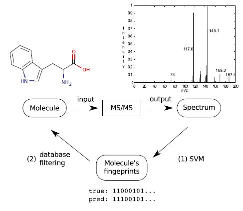
Metabolite identification from tandem mass spectra is an important problem in metabolomics, underpinning subsequent metabolic modelling and network analysis. Yet, currently this task requires matching the observed spectrum against a database of reference spectra originating from similar equipment and closely matching operating parameters, a condition that is rarely satisfied in public repositories. Furthermore, the computational support for identification of molecules not present in reference databases is lacking. Recent efforts in assembling large public mass spectral databases such as MassBank have opened the door for the development of a new genre of metabolite identification methods.
We introduce a novel framework for prediction of molecular characteristics and identification of metabolites from tandem mass spectra using machine learning with the support vector machine (SVM). Our approach is to first predict a large set of molecular fingerprints of the unknown metabolite from salient tandem mass spectral signals, and in the second step to use the predicted fingerprints for matching against large molecule databases, such as PubChem (see Figure 1). We demonstrate that a set of molecular fingerprints can be predicted with high accuracy, and that they are useful in de novo metabolite identification, where the reference database does not contain any spectra of the same molecule.
Fingerprints prediction
We consider fingerprints prediction as a set of binary classification problems where the input is the mass spectra and the output is the fingerprints. We define a spectrum as a set of $k$ peaks $\chi = \{ \mathbf{x}_{1}, \ldots, \mathbf{x}_k \}$ where $\mathbf{x}_{i} \in \mathbb{R}^{2}$. Each peak $\mathbf{x}_{i}$ is a 2-dimensional tuple including the mass of the peak and the corresponding normalized intensity, denoted as $\mathbf{x}_{i} = (mass_{i},int_{i})^{T}$. Our goal is to find the stable patterns between the mass spectrum $\chi \in \mathbf{X}$ and a set of $m$ fingerprints $\mathbf{y} = (y_{i})_{i=1}^{m} \in \mathbf{Y}, \mathbf{Y}=\{0,1\}^{m}$, i.e. a function $f:\mathbf{X} \rightarrow \mathbf{Y}$.
Constructing the kernel is a critical step in SVM. A mass spectrum kernel $K:\mathbf{X} \times \mathbf{X} \rightarrow \mathbb{R}$ implicitly defines a feature mapping $\phi: \mathbf{X} \rightarrow \mathcal{H}$ where $\mathcal{H}$ is Hilbert space such that $K(\chi,\chi^{\prime}) = \langle \phi(\chi),\phi(\chi^{\prime}) \rangle$.
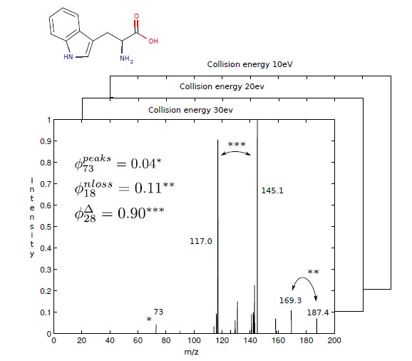
We mainly consider three types of features which all of our kernels represent. The original peaks mass $\phi_{peaks}$ are fragments directly recorded on mass analyzer. This feature is the most simple and useful information we should use. The mass difference between product ions and precursor (mother) ion $\phi_{nloss}$ are included as the complementary information. The difference between every ions (both in first and second stages) $\phi_{diff}$ are extension of the $\phi_{nloss}$. The three features are shown at Figure 2.
The features are employed in two families of mass spectral kernels for SVM classification: an integral mass accuracy kernel and a high mass accuracy kernel, where the peaks conform a gaussian mixture model densities.
Integral mass kernel
The integral mass kernel rounds the mass of peaks to its nearest integer. We explicitly construct the feature space which is a vector of peak intensities. Function $\phi_{peaks}$ defines a feature mapping $\phi: \mathbf{X} \rightarrow \mathbb{R}^{d}$ where $d$ is the upper integer bound for all the peaks in the data set. The $\phi_{peaks}(\chi) = (\phi_{peaks}(\chi)_{i})_{i=1}^{d}$ for $i = 1 \ldots d$, where
$\phi_{peaks}(\chi)_{i} = \sum_{(mass,int)\in\chi}\delta_{i\pm0.5}(mass)\cdot int$, and $\delta_{i\pm0.5}$ is an indicator function,which returns 1 if $i-0.5 < mass < i + 0.5$, and $0$ otherwise.
In tandem mass spectrometry, the precursor ion is selected in the first stage, and it fragmented further in the second stage. The neutral loss feature depicts the mass differences between product ions and the precursor ion, denoted as $\phi_{nloss}(\chi) = (\phi_{nloss}(\chi)_{i})_{i=1}^{d^{\prime}}$, $d^{\prime}$ is the upper integer bound for neutral loss in the data set with
$\phi_{nloss}(\chi)_{i} = \sum_{(mass,int)\in\chi}\delta_{i\pm0.5}(prec(\chi)-mass)\cdot int$
and the $prec(\chi)$ indicates the precursor mass of a molecule mass spectra $\chi$ and $\delta$ is the same indicator function as above. Several peaks may share the same neutral loss due to the very close mass and we add the intensities of such peaks as the value of $i$th dimension in the feature vector.
We expand the idea of neutral loss to mass differences between every peak ions and can think of it as a secondary fragmentation information. We take the rounded mass difference as the index in the feature vector and the product of two peak intensities as the value in that dimension. Thus the $\phi_{diff} = (\phi_{diff}(\chi)_{i})_{i=1}^{d^{\prime \prime}}$ with
$(\phi_{diff}(\chi)_{i}) = \sum_{\substack{(mass,int) \in\chi \\ (mass^{\prime},int^{\prime}) \in \chi}} \delta_{i\pm0.5}(mass-mass^{\prime}) \cdot int \cdot int^{\prime}$
and the $\delta$ is the indicator function defined as before and $d^{\prime \prime}$ is the upper integer bound for peak differences in the data set. The notation for $diff$ feature in Figure 2 is using $Delta$.
Thus the kernels for these three features are defined as:
$ K_{peaks}(\chi,\chi^{\prime}) =\langle \phi_{peaks}(\chi), \phi_{peaks}(\chi^{\prime}) \rangle $
$ K_{nloss}(\chi,\chi^{\prime}) =\langle \phi_{nloss}(\chi), \phi_{nloss}(\chi^{\prime}) \rangle$
$ K_{diff}(\chi,\chi^{\prime}) =\langle \phi_{diff}(\chi), \phi_{diff}(\chi^{\prime}) \rangle$
Addition of kernels represents the feature concatenation. So besides those three independent features, we propose three which defined as follows:
$ K_{peaks+nloss} = K_{peaks} + K_{nloss} $
$ K_{peaks+diff} = K_{peaks} + K_{diff} $
$ K_{full} = K_{peaks} + K_{nloss} +K_{diff} $
To illustrate the effect of addition of kernels, the $K_{full}$ is equal to a feature space $\phi_{full} = (\phi_{peaks};\phi_{nloss};\phi_{diff})$. Polynomial kernels can easily be obtained by applying a polynomial function to the kernel matrix. We tested both linear kernel and quadratic kernel in our experiment.
High resolution mass kernel
The explicit feature representation of the discrete kernel allows direct inspection of the feature weights. However, it rounds all peaks to a nearest integer value. Unique peaks with same rounded mass are erroneously binned together. We can expand the feature space by narrowing the bin widths, however this introduces an alignment problem in the dot product
We assume a probability distribution $p(\chi)$ over a mass spectrum $\chi$ so that the kernel function for two mass spectra becomes kernel function for two probability distributions, $K(\chi,\chi^{\prime}) \equiv K(p,p^{\prime})$. Then we utilize a probability product kernel.
We model the probability $p(\mathbf{x}_{i})\sim \mathbf{N}(mass_{i},\Sigma)$ over the peak $\mathbf{x}_{i}$ of mass spectrum $\chi$ and assume zero covariance between mass and intensity by setting
$ \Sigma = \left[ \begin{array}{cc} \sigma_{mass} & 0 \\ 0 & \sigma_{int} \end{array} \right] $
The probability product kernel for two dimensional gaussian kernel is:
$ K(\chi,\chi') = K(p,p')= \int_{\mathbb{R}^2} p(\mathbf{x}) p'(\mathbf{x}) d\mathbf{x} = \int_{\mathbb{R}^2}\frac{1}{k}\sum_{i}^{k}p_{i}(x_{i})\cdot \frac{1}{k^{\prime}}\sum_{j=1}^{k^{\prime}}p_{j}(x_{j}) d\mathbf{x}$
$= \frac{1}{k} \frac{1}{k'} \sum_{i,j}^{k,k'} \frac{1}{2\pi |\Sigma|^{\frac{1}{2}} |\Sigma'|^{\frac{1}{2}} |\Sigma_{\dagger}|^{\frac{1}{2}} } \cdot \exp \left( -\frac{1}{2} \left( \mathbf{x}_i^T \Sigma^{-1} \mathbf{x}_i + \mathbf{x}_j'^T \Sigma'^{-1} \mathbf{x}_j' + \mathbf{x}_{\dagger}^T \Sigma_{\dagger}^{-1} \mathbf{x}_{\dagger}\right) \right), $
where $\Sigma_{\dagger} = \Sigma^{-1} + \Sigma'^{-1}$, $\mathbf{x}_{\dagger} = \Sigma^{-1} \mathbf{x}_i + \Sigma'^{-1} \mathbf{x}_j'$, and $\mathbf{x}_i \in \chi$ and $\mathbf{x}_j'\in \chi'$, and $\mathbf{x}_{i}=(mass_{i},int_{i}) \in \chi$ and $\mathbf{x}_{j}=(mass_{j},int_{j}) \in \chi^{\prime}$.
We compute the feature class specific kernels $K_{peaks}$, $K_{nloss}$ and $K_{diff}$ as before and derive the three more combined kernels and polynomial kernels as integral mass kernel does.
Metabolites identification
The predicted fingerprints can be used as a way of identifying metabolites by querying the predicted fingerprints against some molecule database.
Having predicted fingerprints and fingerprints database at hand, we need to choose a scoring system to sort all the molecules in fingerprints database for a query. We suggest a probability measurement which takes the variety of accuracy into consideration.
It is a natural idea that we only consider the molecules with similar mass of the querying sample. Thus we first do a mass filtering which reduce the candidates molecules to a subset of the whole molecular database.
Given the cross validation accuracy $\mathbf{p}=(p_{i})_{i=1}^{m} \in \mathbb{R}^{m}$ vector over $m$ fingerprints $\mathbf{y}=(y_{i})_{i=1}^{m}$, we can define the probability of an arbitrary fingerprints vector $\mathbf{y}$ against the correct fingerprints $\mathbf{y}^{\ast}$ with the prediction model $\mathbf{p}$ follows a Poisson-Binomial distribution $\mathbf{y}|\mathbf{y}^{\ast} \sim \mathbf{PB}(\mathbf{p})$ with probability mass function (pmf)
$ p(\mathbf{y}|\mathbf{p},\mathbf{y^{\ast}}) = \prod_{i=1}^{m}p_{i}^{1-|y_{i}-y_{i}^{\ast}|}(1-p_{i})^{|y_{i}-y_{i}^{\ast}|}. $
Based on the pmf function, the probability for a predicted fingerprints vector $\hat{\mathbf{y}}$ is derived as $p(\hat{\mathbf{y}}|\mathbf{p},\mathbf{y}^{\ast})$. We compute the probabilities for every molecules after mass filtering in the database. If the predicted molecule is in the database, it should be ranked as the first among all the molecules since the largest probability is obtained when the molecule fingerprints is exactly the same as the correct molecule. Thus the rank of the predicted fingerprints compare to the other molecules in some database gives us how accurate our prediction is.
In real identifications, the rank of the probability of correct fingerprints given the $\mathbf{p}$ and $\hat{\mathbf{y}}$, i.e. $p(\mathbf{y^{\ast}}|\mathbf{p},\hat{\mathbf{y}})$ depicts how far between our prediction and the real molecule. Noticing that the expected ratio of predicted correct fingerprints is the mean $\frac{1}{m}\sum_{i}^{m}p_{i}$ and $p_{i} \geq 0.5$ which simply means our prediction should and actually is always better than predicting with the majority class and it actually is.
Package usage instruction
We also have a software package avaliable in sourceforge
We maintain two type of package. If you do not have OpenBabel-2.3.0 and LibSVM and not willing to install them, you can download our CDE package. Otherwise, you can download a much smaller standard package which you have to provide the OpenBabel path and LibSVM path as arguments. The related paper Metabolites identification and fingerprint prediction via machine learning has more detail about the methods.
To unzip the packages, you can use following scipt:
tar -zxvf package-name
CDE package usage instruction
The latest version of CDE package is at here:CDE-FingerID-1.2.tar.gz
To run the programme, follow the instructions below.
- After unzipping the package, go to the
'./cde-root/home/fs/hzshen/mass_classification/fingerid-code/'folder. - Putting your training mass spectra and testing spectra into the
train_dataandtest_datafolders. The file should be in the MassBank format. We have sample training data and testing data in the folder. - Setting the arguments in fingerid.cfg Default values are there for all parameters. By using CDE, users do not need to provide libSVM path and OpenBabel path.
- Run the program as
./fingerid-run.cde - Search result are written in
search.res. If validate is set to True in the main module, a filevalidate.reswill also be there. Validate.res contains 3 rows: First row records the ranks of the correct molecules; Second row records search time for querying molecular database; Third row records the number of candidates after mass filtering.
Standard package usage instruction
The latest version of standard package is at here:FingerID-1.2.tar.gz
To run the programme, you need to install OpenBabel-2.3.0 and LibSVM and then follow the instructions below. If you do not have OpenBabel-2.3.0 and LibSVM, you can download CDE fingerid package.
- Putting your training mass spectra and testing spectra into the
train_dataandtest_datafolders. The file should be in the MassBank format. We have sample training data and testing data in the folders. - Setting the arguments in fingerid.cfg. You have to provide OpenBabel-2.3.0 and LibSVM path.
- Run the program as
./fingerid-run - Search results are written in
search.res. If validate parameter in the main.py is set to True in the main module, a filevalidate.reswill also be there. Validate.res contains 3 rows: First row records the ranks of the correct molecules; Second row records search time for querying molecular database; Third row records the number of candidates after mass filtering.
The validate.res will contain useful information only if there are database IDs for the test data and you are searching the same database. For example, we have kegg ligand compound ID in the sample test data and we are searching kegg ligand database by default.
Detailed description of avaliable arguments can be found in the main.py in the package. The kernel computation and SVM training may cost hours depending on the data size.
Database extension
Users can extend the molecular database to any database, e.g. PubChem, if parse the data to specified format as in kegg_mass and kegg_fp.dict. But now we only support validation of the search on Kegg or PubChem (SEARCH_KEGG and SEARCH_PUBCHEM parameters in fingerid.cfg)
kegg_mass contains n*2 matrice where n is the number of entry for some molecular database and the first row is the id for the database entry and the second row is the exact mass of that entry.
Example:

C00001 18.0106

C00002 506.9957

C00003 664.1169

C00004 665.1248

C00005 745.0911

C00006 744.0833

...              ...
Kegg_fp.dict is the python dict ( {"C00001":"0100110101010101010100....","C00002":"11010111000010101010...",...} ) taking database id as the key and corresponding fingperprints as the value. It's a binary file and can be loaded into memory, for instance, by pickle module. You can creat your own dict by the following python code:
f = open("kegg_fp.dict","wb")

pickle.write(f)

f.close()
Notice that the kegg_fp.dict with this relase contains the fingerprints generated by OpenBabel-2.3.0 so to performe identification with this database, you have to use the same version of OpenBabel, that is 2.3.0. The fingerprints may be different in different version. If you are using another version of OpenBabel, you have to rebuild the kegg_fp.dict using your version of OpenBabel.
When you creat your own fingerprints dict, please use the FP3, FP4 and MACCS fingerprints (all together 528 fingerprints) in OpenBabel to make the fingerprints in dict and in the prediction comparable.