SAT-NeRV: SAT-based Neighborhood Embedding Retrieval for Visualization

This is an online supplement to the paper:
Kerstin Bunte, Matti Järvisalo, Jeremias Berg, Petri Myllymäki, Jaakko Peltonen and Samuel Kaski. Optimal Neighborhood Preserving Visualization by Maximum Satisfiability. Proceedings of 28th Conference on Artificial Intelligence (AAAI 2014), Québec City, Québec, Canada, 2014.

We present a novel approach to low-dimensional neighbor embedding for visualization, based on formulating an information retrieval based neighborhood preservation cost function as Maximum satisfiability on a discretized output display. The method has a rigorous interpretation as optimal visualization based on the cost function. Unlike previous low-dimensional neighbor embedding methods, our formulation is guaranteed to yield globally optimal visualizations, and does so reasonably fast. Unlike previous manifold learning methods yielding global optima of their cost functions, our cost function and method are designed for low-dimensional visualization where evaluation and minimization of visualization errors are crucial. Our method performs well in experiments, yielding clean embeddings of datasets where a state-of-the-art comparison method yields poor arrangements. In a real-world case study for semi-supervised WLAN signal mapping in buildings we outperform state-of-the-art methods.

This side contains a demo implementation, supplementary material accompanying the paper and some weighted MaxSAT instances of varying complexity to test new solvers.

[Download] This software package implements the weighted MaxSAT instance writing code for neighborhood embedding retrieval for Visualization. The demo file generates the benchmark helix data and constructs the neighborhood weight matrix W. The weighted MaxSAT instance is written based on that matrix via wsatnerv.m. Note that the solver is not included in the archive! We used the MaxHS solver provided by (Davies and Bacchus 2013).

If you use any of the algorithms implemented in the package, please cite the paper (Bunte et al 2014) from above.

The authors thank Jessica Davies for providing the MaxHS solver:
J. Davies and F. Bacchus. Exploiting the power of MIP solvers in Maxsat. In Proceedings of the 16th International Conference on Theory and Applications of Satisfiability Testing (SAT 2013), volume 7962 of Lecture Notes in Computer Science, 166-181. Springer, 2013.

This is experimental software provided as is; we welcome any comments and corrections but cannot give any guarantees about the code. If you have any comments or bug reports, please direct them to Kerstin Bunte.

Additional Experiments

Click on the image to enlarge!

Wireless	Faces data sets
Color visualization of WLAN by the 2-stage Isomap (A) and MaxSAT on a 16x32 grid (B). Dots represent the 200 fingerprint vectors, triangles the 38 key points, squares the 66 mapped test points. Similar RSSI vectors are colored similarly. Stars are the recorded geographical positions of the test points; lines connect the mapped and recorded positions.	Top: Olivetti faces with our method and t-SNE. Bottom: UMist faces with our method and t-SNE. For UMist both methods are reasonable, for Olivetti faces ours yields a regular arrangement whereas t-SNE packs some faces overly close near the center.
Gene expression experiments	Coil
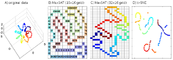
Visualization of a collection of gene expression experiments, with our method and t-SNE. Letters abbreviate manually labeled topics: C (cancer), R (cancer-related), H (HIV), A (cardiomyopathy) and M (malaria).	Visualizations of the coil data set with our method A and t-SNE (panel B). After giving user input on images actually being different around the yellow region (panel C), re-run SAT separates the coils. Defects in data cause all similarities not to be visible in the data (E), which the user can fix by giving prior information, after which SAT again finds a good result (F). The neighborhood weights were constructed using the k=2 nearest neighbors in this experiment.

(Weighted) MaxSAT Instances of Varying Complexity

Data set	nb of points	grid size	nb of variables	nb of clauses	cost of optimal solution	MaxHS solver time	download wcnf file
Swissroll	600	32x32	8571697	45745041	0	217584s	[Download]
Olivetti faces	400	32x32	3993513	21305139	6	36287.42s	[Download]
Umist faces	575	32x32	8253505	44048404	0	32120.65s	[Download]
Wireless (38 keys)	540	16x32	5302850	26845185	5.5246	93128s	[Download]
Wireless (38 keys)	540	16x32	2840991	14377482	6.29641	5219.950s	[Download]
Wireless (38 keys)	540	16x32	1532784	7753446	5.27922	907.166s	[Download]
Wireless (38 keys)	540	16x32	602225	3042810	7.51505	425.512s	[Download]

Detailed Encoding

The position of a point x in the grid is determined by the assignment of (C + R) column and row variables enumerated from right (i.e., from the least significant bit) to right (i.e., to the least significant bit): c_C^x, … , c₂^x, c₁^x and r_R^x, … , r₂^x, r₁^x. The neighborhood clauses of the bit-based encoding are represented with clauses as follows:

Recall: If W(x,y)>0, we want x and y to be row, column or diagonal neighbors on the grid. For each point x and for all y such that W(x,y)>0, we introduce the soft clause (RNxy∨CNxy∨DNxy) with weight W(x,y)/2.

Precision: If W(x,y)<0, we want x and y not to be row, column, or diagonal neighbors on the grid. We encode this with the soft clause (PRxy) with weight |W(x,y)|/2.

The propositional formulas of the bit-based encoding are represented with clauses as follows:

CNxy: for all pairs of constraint points (x,y) introduce the following hard clauses: (CNxy∨¬SRxy∨¬ACxy) (¬CNxy∨SRxy) (¬CNxy∨ACxy)	RNxy: for all pairs of constraint points (x,y) introduce the following hard clauses: (RNxy∨¬SCxy∨¬ARxy) (¬RNxy∨ ARxy) (¬ RNxy∨ SCxy)
DNxy: for all pairs of constraint points (x,y) introduce the following hard clauses: (DNxy∨¬ARxy∨¬ACxy) (¬DNxy∨ARxy) (¬DNxy∨ACxy)	PRxy: for all pairs of constraint points (x,y) such that W(x,y)<0 introduce the following hard clauses: (¬PRxy∨¬RNxy) (¬PRxy∨¬CNxy) (¬PRxy∨¬DNxy)
EQxyj for rows: for all pairs of constraint points (x,y) and all row bits introduce the following hard clauses: (¬EQxyj∨¬rxj∨ ryj) (¬EQxyj∨ rxj∨¬ryj) (EQxyj∨ rxj∨ ryj) (EQxyj∨¬rxj∨¬ryj)	EQxyj for columns: Similar to EQxyj for rows but stated over column bit variables instead.
SRx: for all pairs of constraint points (x,y) introduce the following hard clauses (using the EQxy variables for rows): SRxy∨∨j=1R¬EQjxy (¬SRxy∨EQjxy) for all j=1…R	SCxy: similar to SRxy but using the EQxy variables for columns instead.
SRxy: for all pairs of constraint points (x,y) introduce the following hard clauses (using the EQxy variables for rows): SRxy∨∨j=1R¬EQjxy (¬SRxy∨EQjxy) for all j=1…R	SCxy: similar to SRxy but using the EQxy variables for columns instead.
Fixy for rows: for all pairs of constraint points (x,y) and all row bits 1 ≤i ≤R introduce following hard clauses: (¬Fixy∨¬rxk) for all k=1…i-1 (¬Fixy∨ryk) for all k=1…i-1 Fixy∨∨1≤k≤irxk∨¬ryk	Fiyx for rows: for all pairs of constraint points (x,y) and all row bits 1 ≤q i ≤q R introduce following hard clauses: (¬Fiyx∨¬ryk) for all k=1…i-1 (¬Fiyx∨rxk) for all k=1…i-1 Fixy∨∨1≤k≤i ryk∨¬rxk
F_ixy and F_iyx for columns: similar to Fixy and Fiyx for rows. But stated with column bit variables instead.
Aixy and Bixy for rows: for all pairs of constraint points (x,y) and all row bits 1≤i≤R introduce the following hard clauses (using EQxy, Fxy and Fyx variables for rows): ¬Aixy ∨EQixy∨¬rxi∨ Fixy∨∨j=i+1R¬EQjxy (Aixy∨EQjxy) for all j=i+1…R (Aixy∨¬EQixy), (Aixy∨rxi), (Aixy∨¬Fixy) ¬Bixy ∨EQixy∨rxi∨ Fiyx∨∨j=i+1R¬EQjxy (Bixy∨EQjxy) for all j=i+1…R (Bixy∨¬EQixy), (Bixy∨¬rxi), (Bixy∨¬Fiyx)	Aixy and Bixy for columns: similar to Aixy and Bixy for rows but using column bit variables as well as EQxy, Fxy and Fyx variables for columns instead.
ARxy for all pairs of constraint points (x,y) introduce the following hard clauses using Axy and Bxy variables for rows: ARxy∨∨i=2R(¬A_ixy∨¬B_ixy) (¬ARxy∨A_ixy) for all i=2…R (¬ARxy∨B_ixy) for all i=2…R	ACxy: Similar to ARxy using Axy and Bxy for columns instead.
Using the basic encoding points may fall onto the same position in the grid. In order to prevent that one includes following hard clauses for each pair of points: (¬SCxy∨¬SRxy)

Proof Sketch of Theorem 1

Follows from four observations:
(i) an arbitrary assignment of the row (column) bits r_i^x (c_i^x) for each data point x∈ P and i=1…R (C) corresponds a mapping of P into G (and vice versa);
(ii) an arbitrary assignment of the row and columns bit-variables (r_i^x and c_j^x) of all data points x∈P can be extended to a solution of the MaxSAT instance (satisfying all hard constraints in the instance);
(iii) (recall) any solution to the MaxSAT instance that satisfies (does not satisfy) the soft clause (RN^xy∨CN^xy∨DN^xy) corresponds to a mapping of P into G in which x and y are (not) mapped into neighboring grid positions (and vice versa);
(iv) (precision) any solution to the MaxSAT instance that satisfies the soft clause (PR^xy) must also satisfy the hard constraint PR^xy→(¬RN^xy∧¬CN^xy∧¬DN^xy), and thus (¬RN^xy∧¬CN^xy ∧ ¬DN^xy); thus the solution corresponds to a mapping of P into G in which x and y are not mapped into neighboring grid positions. To the other direction, given any mapping of P into G which does not map x and y to neighboring grid positions, there is a MaxSAT solution corresponding to the mapping which satisfies the soft clause (PR^xy).